www.wallpaperup.com
Have you ever heard of neutral steer, understeer and oversteer? You probably have heard these terms, and you might even know what they mean, but do you know how it happens or what a racing car’s suspension has to do with it? If your answer to the latter question was “well, no…” or something similar, then this post might be useful.
First, let’s make things straight. In this post I will explain neutral steer, understeer and oversteer in terms of steady-state cornering mechanics, in a linear way, i.e. in the elastic range of tyre operation. We will assume sublimit conditions, and the engineering definitions shown here should not be confused with the definitions of understeer and oversteer for behaviour at the limit of tyre grip. I will address full nonlinear car behaviour in a later post, but first things should come first.
Therefore, let us address the subject in a simpler way first, so that the fundamental concepts will be more easily understood. This approach is called by the gods of Vehicle Dynamics, William and Douglas Milliken, in their legendary book Race Car Vehicle Dynamics (if you have not read a single chapter of this book, stop reading this post right now, and go buy yourself a copy, trust me, you will not regret this!) as the “Ladder of Abstraction”. Here one starts with a simpler model based on simplifying assumptions and escalates through it until it gets as close as possible to the complete reality of the functioning race car. Before reading this, I suggest you read my previous post “The Absolute Guide to Racing Tyres – Part 1: Lateral Force”.
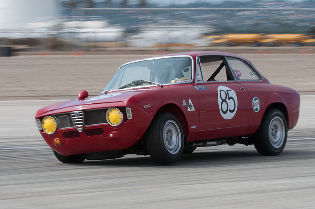
A little bit of understeer! 🙂 SBGrad’s Flickr
The Rudimentary Car Model (Bicycle Car Model)
To explain the physics involved in neutral steer, understeer and oversteer, let us define our simplified model of a race car. This is required in order to generate simpler equations (yes, there will be equations, but I promise to keep them to an elementary level to Engineering student). The model is called a “bicycle car model” in most of the literature on vehicle dynamics, and the name will be repeated here. Before starting to define the model, it is good practice to define the vehicle rotational motion. Figure 1 explains.
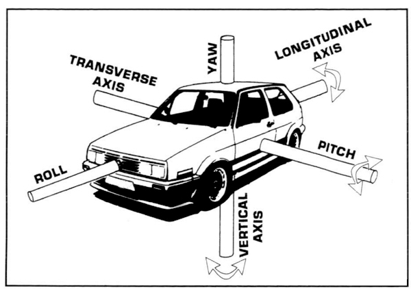
FIGURE 1. Yaw, pitch and roll motions defined along the principal axes of movement. (retrorims.co.uk)
For this model, we will make the following assumptions:
-
- The steer angles of left and right wheels are assumed to be equal, and the front and rear axles are treated as single tyres (hence the name of the model) that generate a lateral force equal to the sum of left and right tyres on each axle. This also presumes that there is no lateral load transfer on the car;
-
- Also, there is no longitudinal load transfer;
-
- No pitch or roll motions, as defined on figure 1;
-
- The tyres operate in the linear (elastic) range. This requires that the car goes through a corner under low lateral accelerations (lateral acceleration is high enough to generate slip angles, but low enough to keep the tyres from reaching the transitional range of operation;
-
- The car is in a constant forward speed (steady-state);
-
- There are no aerodynamic effects present;
- The model assumes the driver uses “position control” of the car. This means that the restraints imposed to control the car directional behaviour will be only placed in the form of steering displacements. This is opposed to “force control”, where the restraints are imposed in the form of steering torques. In real world, the race driver senses both, position and torque feedback from the steering system, in unknown proportions.
For this model, the only input is the steering angle δ and the two outputs are lateral velocity v and yaw velocity or yaw rate r. Figure 2 shows a graphical representation of the model.
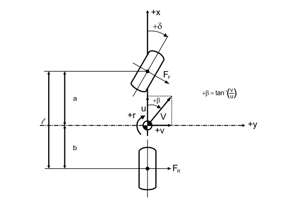
FIGURE 2. Bicycle car model. (MILLIKEN & MILLIKEN, Race Car Vehicle Dynamics – Adapted).
When a car goes through a corner, it passes through three stages, called transient corner entry, steady-state cornering and transient corner exit. They happen as follows:
-
- In the corner entry, both v and r are increasing in time, and thus, their time-derivative is positive (remember v is the lateral velocity, not to be confused with the forward velocity V of the vehicle).
-
- In the steady-state cornering phase, the lateral and yaw velocities are constant, and their time-derivative are zero.
-
- During corner exit, v and r are again decreasing, before turning into zero when the car hits a straight.
These phases might have different durations depending on the type of corner and other characteristics. For example, in long corners with large radius, such as the 130R in Suzuka Circuit, the steady-state phase may be relatively longer than the other phases, while in tight-turn as the Grand Hotel hairpin, in Monaco, the transient phases are much longer. In this post, I will address only steady-state phase, but I will refer to transient cornering in later posts.
Low Speed Cornering
To begin our analysis, let’s consider the case of our bicycle model car going through a corner very slowly, such that there is no relevant lateral acceleration. Because of that, there are no slip angles developed in the tyres, so that they follow the exact geometric path imposed by their rolling motion (purely geometric turning).
In this case, the radius of turn (the distance from turn center to the centre of gravity of the car), R, is dependent only on the wheelbase l of the car (the distance between front and rear axles centrelines) and the steering angle δ.
We define now, the Ackermann Steering Angle (or the wheelbase angle), as the geometric steer angle required for a car of wheelbase l to go through a turn of radius R, at slow speeds, such that external forces due to lateral accelerations are negligible. If we use the small angle approximation, and the Ackermann Steering Angle is given in radians, then, δ=l/R. Figure 3 represents this angle.
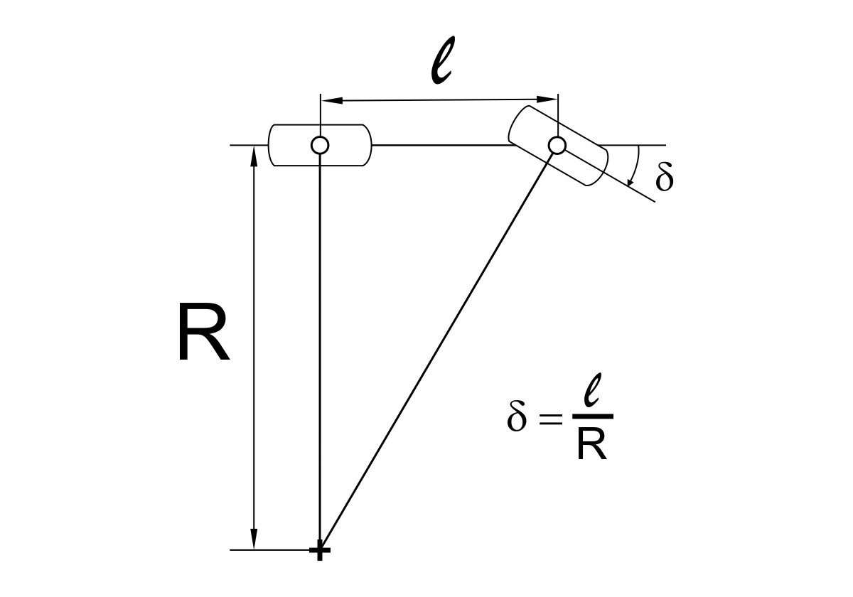
FIGURE 3. Ackermann Steering Angle.
Neutral Steer Car in Steady-State Cornering
Let’s now analyse our model car in a higher forward velocity. The assumptions are as stated in the model description, and now we have lateral acceleration high enough to generate slip angles on the tyres, but not as high to take the tyres beyond their elastic range of operation.
For this case, a car with 50/50 longitudinal weight distribution, such that the normal forces are equal on front and rear tyres. In addition, we consider that both tyres have equal cornering stiffness. Figure 4 illustrates this car on corner under a lateral acceleration ![]() .
.
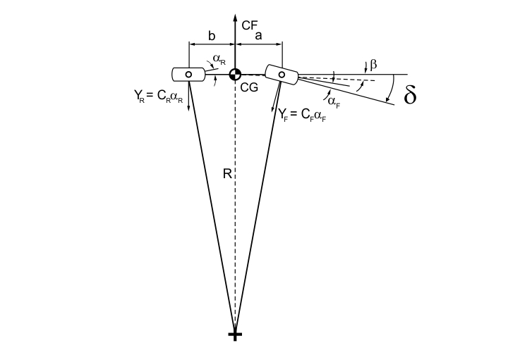
FIGURE 4. Neutral steer car through a steady-state corner.
Now an inertial force (centrifugal force) arises, pushing the car outside the corner. If we take the force and moment equilibria about the centre of gravity (CG) of the car, we will find that the lateral forces developed by both tyres should be equal, and since their cornering stiffness are also equal, then they should have the same slip angle. The equations are shown below.


Before making conclusions about this analysis, let us define the vehicle slip angle or attitude angle, β as the angle between the chassis centreline at the CG and the tangent to the actual path the car is taking. This rotation establishes the attitude of the car with its path. Now, let us make some observations about the analysis.
-
- The same steer angle is required to negotiate the turn, regardless of the speed;
-
- The vehicle slip angle is obtained by rotating the entire vehicle by the amount
 (rear slip angle). This is because in this simple model, the wheel plane of the rear tyre is always parallel to the chassis longitudinal centreline;
- The vehicle slip angle is obtained by rotating the entire vehicle by the amount
- In this situation, the rear wheel will travel at a smaller turn radius than the front;
The rotation that gives rise to rear slip angle also causes some slip angle to be developed on front tyre. For the configuration presented in this case (50/50 longitudinal weight distribution and  ) the slip angle required to produce the force and moment equilibrium is obtained entirely from the rotation of the vehicle during the development of rear slip angle.
It is important to notice that slip angles on front tyres arise from vehicle rotation and steer angle, but in the case presented the component from steer angle is zero. This happens because, even if the steer angle is increased, the gain in lateral force will increase the slip angle on rear tyres, also increasing the vehicle attitude angle, and hence, the front slip angles.
For this configuration, the steer angle δ required to negotiate the turn is equal to the Ackermann Steering Angle,  . All in all, the vehicle will follow the exact geometric path determined by the wheel planes, and the required steer angle will be independent of speed or lateral acceleration.
Thus, we can define this type of handling configuration as neutral steer (NS) because it will neither “understeer” nor “oversteer” the intended path established by Ackermann Steering Angle, as lateral acceleration is increased.
If we do a skid pad test, where the vehicle goes through a large radius circle, with its velocity being discretely increased each time the car travels the entire circle, but without putting the tyres out of their linear range, and plot the required steer angle versus the lateral acceleration of the car, we would obtain a graph like the one shown in figure 5.
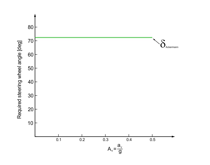
FIGURE 5. Constant radius skid pad test plot for a neutral steer car, for the linear range of the tyres.
From the graph, we can see that the steer angle is kept constant, as lateral acceleration is increased. It is important to notice that this is a rather idealized behaviour. In a real car close to a NS behaviour, the steering angle would either increase or decrease at higher accelerations. This variation will be very small, though, and the deviation from ideal NS behaviour could be neglected.
With increasing lateral acceleration, the slip angles will also increase, but in a NS car, they would increase equally, such that the vehicle path would be determined only by the steering angle. Mathematically, this means that the gradients of front and rear slip angles with lateral acceleration is equal for the entire range of lateral accelerations that the vehicle will exposed to.
Understeer Car in Steady-State Cornering
Let’s now have our model car with one major modification compared to the previous case. Now the CG is moved towards the front of the car, such that its distance to the front axle is one third of the wheelbase (here, 1/3 is just a number that will simplify calculations, the point to keep in mind is that the weight of the car is shifted to the front). This displacement of the CG will now make the front/rear (F/R) weight distribution to be 66%/33%. The front and rear tyre cornering stiffnesses will still be the same. The lateral acceleration ![]() is the same of the previous case.
is the same of the previous case.
If the force and moment equilibria are taken for this case, we will see that the lateral force generated by the front tyre will be twice the one developed on the rear tyre.
Since the cornering stiffnesses are equal, the front slip angle ![]() must be twice the rear slip angle
must be twice the rear slip angle ![]() .
.

Hence the lateral accelerations are the same, we can use the total weight of the car, W, and the slip angle of the NS case,  (same front and rear), to do the following calculations:

Let  be the turn radius for this case. For this to be equal to the turn radius of the NS case, the vehicle attitude angle β is smaller, due to the reduction in the rear slip angle. Thus, the component of the front slip angle generated by this rotation is smaller. This is shown in figure 6.
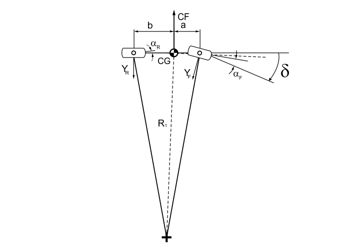
FIGURE 6. Understeer car through a steady-state corner.
Comparing to the NS case,  of the component of front slip angle due to body rotation is lost, and this must be compensated by an increase in steer angle. However, an extra increase on slip angle is needed in order to give the required front slip angle value of
 ![]() . This also must be generated by an increase in steer angle.
. This also must be generated by an increase in steer angle.
To sum up, the required steer angle to negotiate the turn in this case is increased by  in relation to the NS car. This increase comes from the difference between front and rear angles.
One important thing to notice, is that slip angles will define the actual path taken by the car – the front slip angles trying to steer the car away from the turn, while the rear slip angle tries to bring the vehicle into the turn. The net steering effect is given by  , towards the outside of the corner. The total steering angle is given by:

The handling in this case is called understeer (US) because the vehicle tends to “understeer” the path established by the Ackermann Steering Angle, when lateral acceleration is increased. Figure 7 shows the constant radius skid pad plot of an understeer car. Here, it is possible to see that the required steering angle to keep a constant radius increases with lateral acceleration. The slope of curve is called understeer gradient of the car, and can be used to quantify either understeer or oversteer (when gradient is negative) of the car.
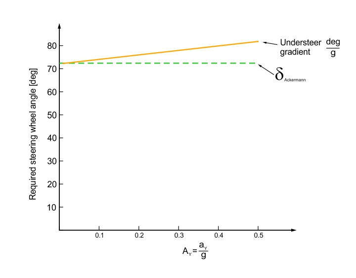
FIGURE 7. Constant radius skid pad plot of an understeer car.
So far, we have defined understeer in terms of weight distribution and tyres cornering stiffnesses, but this can be generalized by observing that any design change that would affect the front and rear slip angles increase rate, would affect the understeer/oversteer balance of the car. The difference  is what will define how the car will behave. These gradients are affected by other parameters, mainly those involved with the suspension of the vehicle, and you will see three of these factors at the end of this post.
Oversteer Car in Steady-State Cornering
Now imagine that we shift the CG of our model car to the rear, such that its distance from the rear axle centreline is  (again one third of the wheelbase is just for mathematical reasons). Analogous to the US case, the F/R weight distribution is now 33/66. The cornering stiffnesses remain the same. Again, taking force and moment equilibria, we should have:
Doing the same calculations done for the US car’s slip angles in respect to the NS slip angles (), we should now obtain:
Now the effect of the rotation of the chassis will add to the front slip angle (as noted in US example), and this must be reduced by decreasing the steering angle. A further decrease of in front slip angle must be introduced, in order to bring ![]() to the required value of . This is also achieved by a reduction in steering angle. Figure 8 shows the model for this case.
to the required value of . This is also achieved by a reduction in steering angle. Figure 8 shows the model for this case.
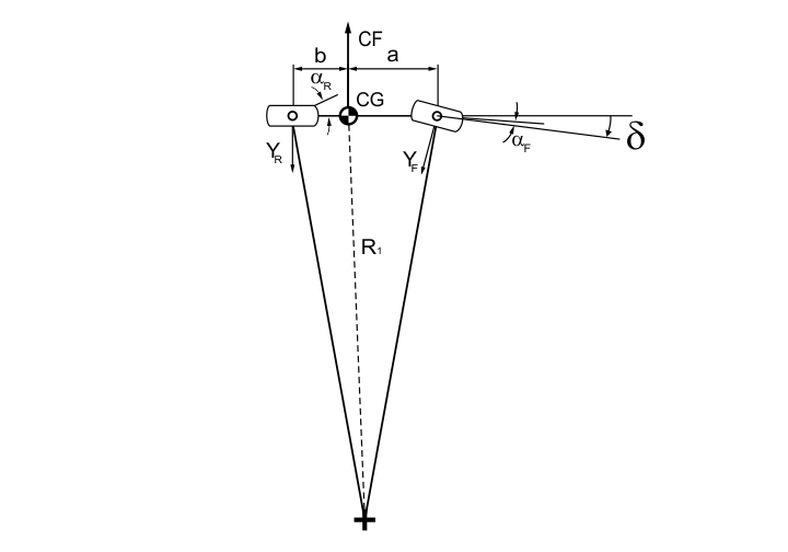
FIGURE 8. Oversteer car through a steady-state corner.
The required steering angle for this oversteer vehicle is given by:
Again, the net steering effect will be given by the difference between front and rear slip angles. Since, this time rear slip angles are larger, we will have the rear axle being the dominant one, tending to push the car into the turn. This means that an oversteer car will corner with a more nosed-in attitude, but with smaller steering angle in relation to NS and US cars.
We therefore define this handling case as oversteer (OS) because the vehicle tends to “oversteer” the path established by the Ackermann Steering Angle, when lateral acceleration is increased. Figure 9 shows the constant radius skid pad plot for an oversteer car. Now the slope of the curve is negative, indicating that steering angle is reduced when lateral acceleration increases.
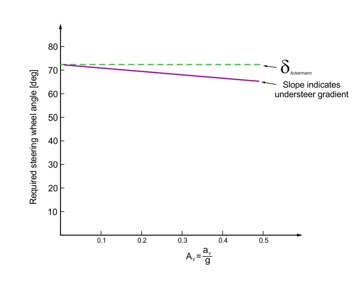
FIGURE 9. Constant radius skid pad plot of an oversteer car.
3 Ways in Which Suspension Affects Understeer and Oversteer
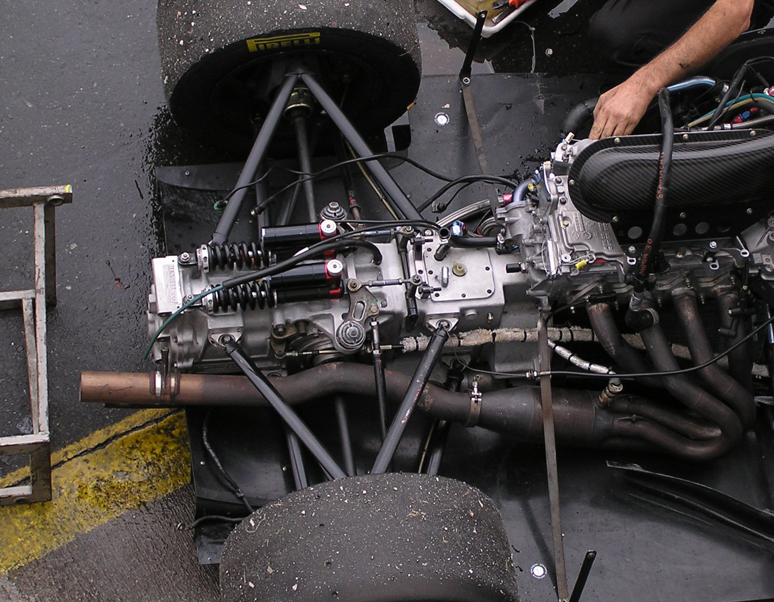
commons.wikimedia.org
As stated before, any factor that alters the way slip angles vary with acceleration will be reflected on the understeer/oversteer balance of the car. The key here is to understand that the difference between slip angle gradients in respect to lateral acceleration is what will make the net steering effect. And suspension is a major controller of those parameters. Let us see how.
1. Roll Moment Distribution
In the previous post about the generation of lateral force in a racing tyre, I talked about what is called the tyre load sensitivity (the tendency of the tyre to generate higher lateral forces in a smaller rate with increasing vertical load) and how it is related to the load transfer in an axle. As previously said, when there is load transfer in an axle, the total lateral force generated in this axle is smaller.
Now, if we have higher lateral load transfer (LLT) in an axle in relation to the other, it will contribute to either understeer or oversteer, depending on which axle has a higher LLT.
I addressed the mechanics of lateral load transfer in detail, in another post. For now, you just need to know that the suspension affects lateral load transfer in three major ways:
-
- Roll Center height – in a nutshell, the roll center is the point where the lateral force is transmitted from the sprung mass (all the mass of the car that is supported by the suspension) to the unsprung mass (all the mass of the car that is not supported by the suspension itself). The roll center position is controlled by suspension geometry, and basically, the higher the roll center, the larger will be the lateral load transfer (this is not the case for 100% of the cars, but it works for most of them, more on that in the aforementioned post about lateral load transfer);
-
- Roll Moment distribution – simply put, the roll moment is the moment that makes the vehicle roll to the outside of the corner when under significant lateral accelerations. As it is easy to notice, the higher the roll moment, the higher the LLT. The key factor here is that roll moment is different for the front and rear axles, and hence this will interfere with oversteer and understeer. The roll moment in an axle is proportional to the stiffness in roll of the suspension of that axle. This stiffness, called roll rate, is affected by spring rates and the lateral distance between them, or equivalently to the track size of the vehicle.
- Unsprung Weight – the unsprung weight is also, well, weight. Hence, under lateral acceleration, it will cause a centrifugal force that will be applied on the CG of the unsprung weight (which will always be above the ground). This will generate a moment that will also transfer load from the inside tyre to the outside one. Suspension affects it because the weight of suspension is part of the unsprung weight. In general, design changes can’t be made in relation to this aspect, because usually the mass of components in a racecar is already reduced to the minimum possible.
2. Camber Change
First, the definitions. Camber is the angle of inclination of the wheel plane in respect to a vertical plane going through the longitudinal centreline of the car. It is defined as negative when the top of the tyre is pointing towards the inside of the car and positive when the opposite happens.
Camber will produce a lateral force called camber thrust. Camber angle will produce much less lateral force than slip angle, and hence, this effect is secondary. However, the most important interaction between camber and the generation of lateral force is the effect of the former on tyre contact patch.
When the chassis rolls in a corner, an amount of camber equal to the roll angle is induced on the tyres. This results in positive camber on the outer wheels and negative on the inner ones. This configuration reduces the tyre contact area, and hence must be counteracted. Engineers do this either by using negative static camber, as shown on the figure below, or by intentionally inducing camber variation with suspension travel opposite to the one induced by chassis roll. The amount of predefined camber wheel has a great impact on the lateral force produced by the front and rear tyres, and hence, significantly affects the balance of the car.
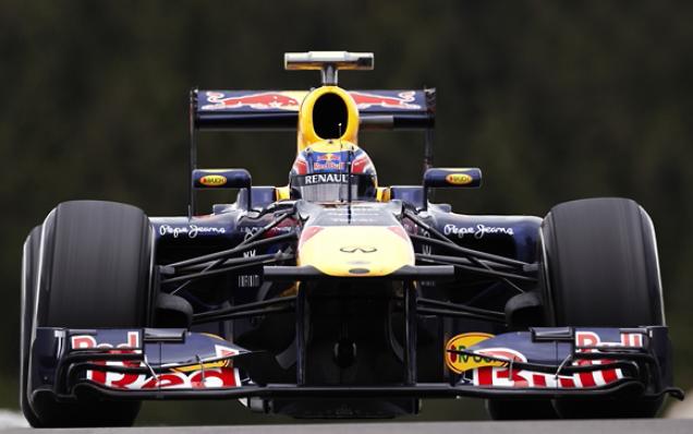
FIGURE 10. Red Bull RB9, with high negative camber on front tyres. (PulpAddict.com)
3. Roll Steer
Roll steer is the variation of tyres (front and rear) steer angles when the chassis roll. The suspension kinematics will be responsible for that, and it can be controlled to contribute to either understeer or oversteer, as the steer angle directly affects handling by altering slip angles.
I hope have enjoyed this article. On the next post on vehicle dynamics, I will address lateral weight transfer, and will explain the mechanisms through which it happens. You don’t want to miss that, do you? Then, please subscribe to our e-mail list below, to receive an e-mail when I post anything here on Racing Car Dynamics. Plese don’t forget to share your thoughts on this article on the comments below! 😉