Photo: Youtube Video (Infiniti Europe’s channel)
If you are a keen motorsport fan, or a Vehicle Dynamics enthusiast, you probably have heard of the use of simulation in racing. On the recent days, the word “simulation” has been more and more on the motorsport media, in all sorts of levels. But do you know how it is used?
With the regulations in all categories and levels of motorsport increasingly pushing teams and companies to reduce costs, track time became strictly limited, and the racing world saw the main tool for vehicle development (testing) having its use severely restricted.
The scenario above created a demand for the improvement of alternative tools that would help to develop the cars. This, together with the increase in computational power at diminishing cost through the years, has contributed to the popularisation of simulation tools in racing.
Simulation is used at many levels of the sport, and its role has increased to the point where teams can figure out a huge part of the setup of the car solely based on this tool. In fact, the team management from Audi declared that 99% of the setup of their cars was determined by lap time simulation in the 2009 DTM season.
Some of the advantages of using simulation are:
- It allows development of systems (e.g. suspension and steering), with a significantly reduced number of required prototypes, thus reducing cost;
- It produces data for multiple configurations without having to physically test the car;
- It produces data channels that cannot, or are difficult to measure on the actual car (e.g. tyre loads, dynamic roll centre locations, camber angles, slip angles, etc.). This channels can also be used to increase the accuracy of math channels for the real car;
- It produces a theoretical performance limit for the car, and allows to investigate how close the driver is taking the car to that limit;
- It can be used to investigate the effects of individual changes on vehicle data, preparing the engineers to know what to expect from the data when that change is implemented on the real car.
One thing that engineers must keep in mind is that simulation is only a tool, and should be used as such. Therefore, the users of this tool must have an understanding of how it works, what it can and what it can’t do.
Also they must have an understanding of vehicle dynamics at the most fundamental levels, in order to make it work properly. An analogy that might help you to understand it better is that of a word processor and a writer. The word processor makes the life of the writer significantly easier. However, it won’t write the book for the writer. A very important engineering principle holds true for the use of simulation (and many other engineering tools):
This means that your simulation results will be as accurate as the parameters input to the software. Also the results from the runs must not be blindly trusted. After the results are obtained from the simulator, they must be validated by comparison with track data.
Wanna know more about the use of simulation in racing?
Then keep reading this article to learn more about:
- What are the different uses of simulation in the motorsport environment;
- What is required to put a race car model together;
- How tyres are integrated to the simulation, and what is the Magic Formula Tyre Model;
- What is required to proper model the race track for lap time simulation purposes;
- What you should pay attention to when using simulation.
Applications of Simulation
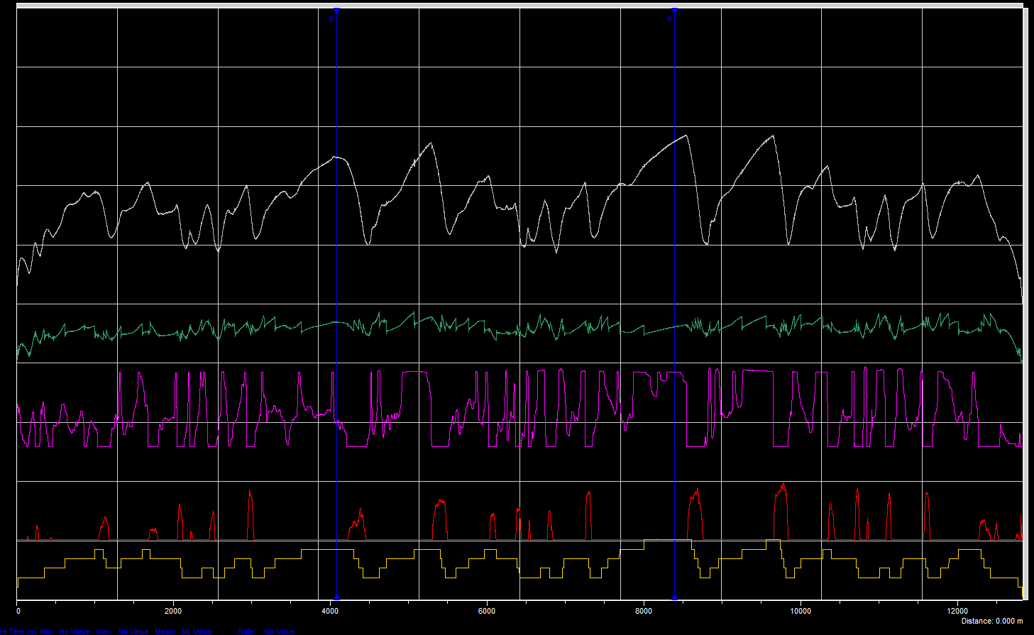
Sample data from simulation.
Several applications for simulation tools are possible at different stages of a race car development. The ones discussed in this post are:
- Suspension kinematics
- Lap time simulation
- Race strategy
Suspension Kinematics Simulation
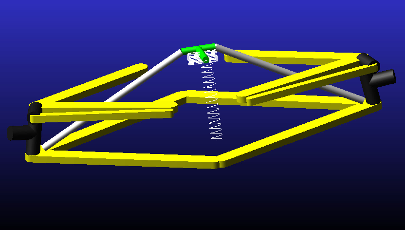
Kinematic model of the front suspension of a Formula Renault 3.5 car.
Simulation of suspension geometry has two main purposes: to support the design of the suspension itself, and to help to create math channels relating to the suspension for the data acquisition software. Generally, suspension geometry simulation packages allow the user to input the three-dimensional coordinates of the suspension pickup points and some other vehicle dimensions, such as wheelbase, track widths, tyre radius and CG height (required for anti-pitch features).
Generally, the following parameters will be outputs of interest:
- Camber angle
- Toe angle
- Caster angle and mechanical trail
- Kingpin Inclination and scrub radius
- Installation ratio (or motion ratio)
- Anti-lift, anti-squat and anti-dive percentages
- Track width change
- Ackermann steering percentage
- Roll centres location
These parameters are generally plotted against wheel travel, ride height, roll angle or steering wheel angle. When the coordinates of the pickup points are not available from the manufacturer, care must be taken when measuring them. The results of the model will be as accurate as the data input to it, and depending on the suspension layout, millimetres can make a huge difference.
Lap Time Simulation
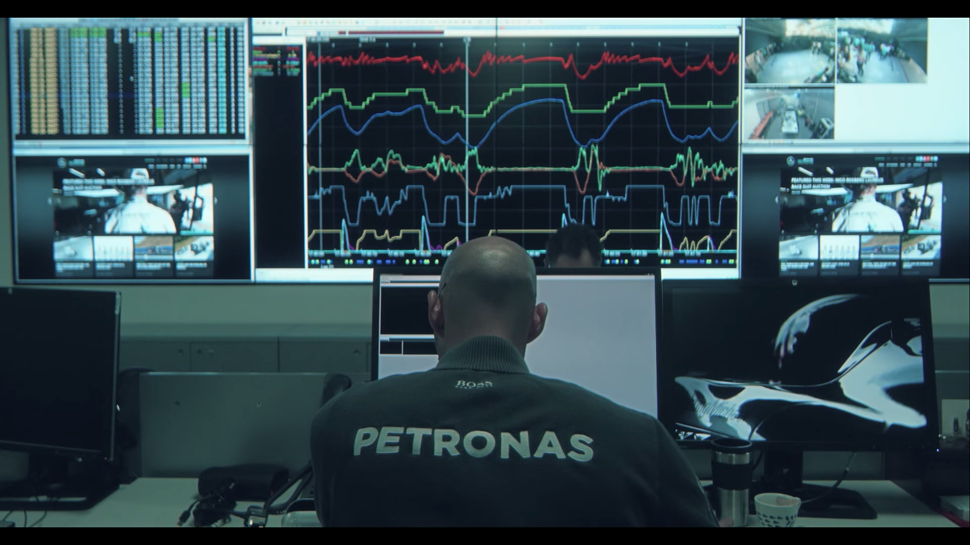
Photo: YouTube video (Mercedes AMG Petronas’ channel)
This is probably the application of vehicle dynamics simulation with most usage in racing. It helps the engineers to increase their knowledge on track-specific performance of the vehicle. Also, lap time simulation allows to test multiple configurations for a particular track and to arrive at the venue with a setup close to optimum together with a clever plan for modifications.
Several strategies are used for lap time simulation, depending on the stage of the development, time and resources available to the team. The following classification is presented in a good part of the specific literature:
Steady-state simulation
This is the most basic level of lap time simulation. Here the vehicle is assumed to be in a state of pure lateral or longitudinal acceleration, i.e., either braking, accelerating or cornering.
This approach has the advantages of ease of calculation, very low computational cost and reduced amount of parameters required (and hence less measurements to be made). The disadvantages of using this simulation strategy are the poor accuracy and the reduced amount of parameters whose effects can be investigated.
Quasi-static simulation, pseudo-static or quasi-steady-state simulation
In this strategy, the circuit is broken down into many corner segments defined by a length and a constant radius, connected together by multiple straight segments. The car is assumed to be in a steady state in each of the segments and the D’Alembert’s principle is applied to find the motion state of the car.
This strategy is useful to provide first insights on wing levels and gear ratios. It’s also very helpful to investigate the effect of variations on grip levels (for example, from changes in weather condition), increase or decrease of engine power, and to get to know the impacts of improvements/worsenings of performance at specific track segments on overall lap time, helping to evaluate setup compromises. Its advantages are the low computational cost and the speed in which results are provided.
The problems with this type of analysis are the negligence of damping and unsprung masses oscillation effects, transient effects such as direction changes and heat build-up on tyres. It also does a poor job on modelling tyre loads, since it can’t capture transient load fluctuations.
Transient simulation
This strategy uses the full equations of motion of the car and integrates them as a function of time. It takes into account the time response of the vehicle, modelling its change of directions (attitude and position) and other important effects such as unsprung mass oscillation and tyre load fluctuation. This strategy demands a controller that takes the role of the driver, representing it in a way to extract the maximum performance of the vehicle.
I will introduce an important distinction from the next strategy. Here I will assume that in a transient simulation the wheels will not move in relation to the body in any direction but the vertical, i.e., no camber, toe, track width changes with wheel travel. This isn’t a distinction that I found on the literature, but the reason why I’m making this distinction will become evident once I present the next strategy.
The advantages of this strategy are the increased accuracy, the possibility of investigating damping effects, and the modelling of transient phenomena. The setbacks are the increased computational cost and the time needed to run the simulations.
Because we are assuming only vertical movement of the wheels, dynamic roll centre positions and suspension geometry effects are disregarded, unless they are modelled through a direct function of wheel travel. This approach is called “the concept suspension”, and is the basis of many vehicle dynamics modelling tools.
Multibody System Simulation (MBS)
The only difference from this strategy to the transient approach presented above is that it models the suspension through parts connected to the chassis, be it through a simplified model such as a swing arm or solid axle with equivalent roll stiffness, or a complex model with bodies representing each of the suspension linkages (linkage model). The reason why I like to use this distinction is because the modelling of the parts of the suspension introduces equations of motion for each component of the system, and constraint equations to restrict the motion of these bodies. Hence, with the multibody system approach the computational cost is much larger, and it takes more time to obtain the results.
There are sublevels to which the suspension can be modelled as a multibody system. The simplest of these levels is called the roll stiffness approach, where the suspension is modelled as a solid axle connected to the body through a revolute joint and a torsional spring/damper that matches the roll stiffness of that end of the car. The most complex model is the linkage approach, where the suspension linkages are modelled exactly as on the actual suspension. If required, bushings might be applied to the model to evaluate the effect of suspension compliance.
Depending on the suspension modelling approach, this can be the most accurate approach, with only the actual car getting more reliable results. The main drawbacks of this strategy are the great demand for computational power, and the longer times to run it.
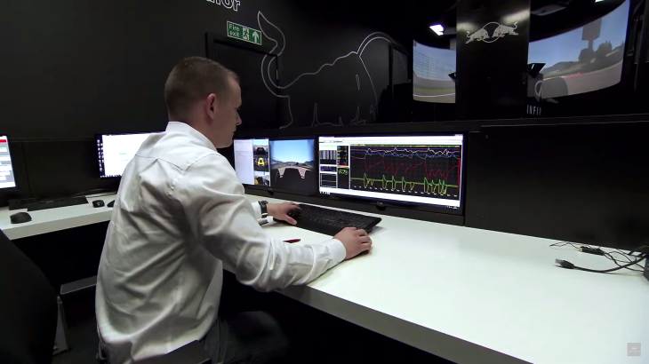
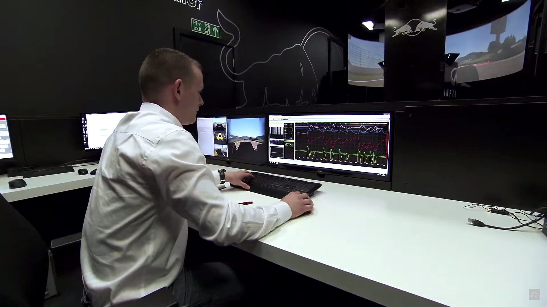
Driver-in-the-Loop Simulation
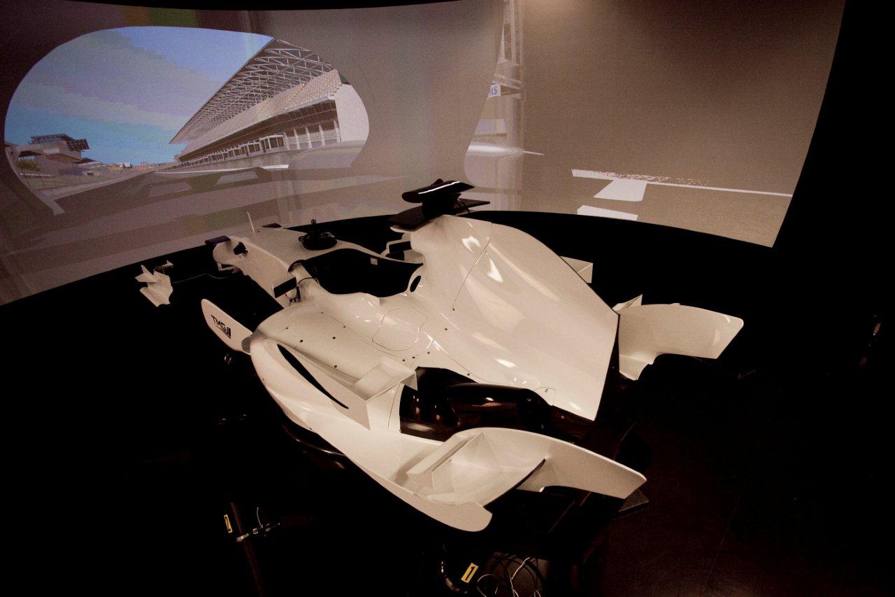
Photo: Toyota Motorsport
Some of the lap time simulation packages don’t integrate a way to model driver behaviour, and assumes that the car will always run on the grip-limit. This may result in a setup that will give the ultimate lap time, but will be undriveable in the real world.
Driver inputs are a very important part in determining the vehicle behaviour. These inputs will depend on the feedback that the driver receives from the car and the track, in the form of the self-aligning moment (a torque that tends to steer the wheels back to a straight position, translating into a feel of heaviness on the steering wheel), vibration perception, and motion cues that will give a perception of the yaw rate of the car.
To help with that, a relatively new technology is getting increasingly greater importance. It’s called driver-in-the-loop simulation. In this type of simulation the vehicle is modelled with standard practices, but instead of using a controller model to produce the inputs to the model (steering wheel angle, throttle, braking and gear change), the actual driver controls the virtual car. The most advanced level of this technology uses motion platforms linked to the dynamic model of the car, and uses inertial forces to “deceive” the vestibular system of the driver in order to provide cues for lateral and longitudinal acceleration. Yaw rate cues are also provided through rotation of the platform, and the system can increase the feel of acceleration through dynamic effects as well.
Examples of the application of motion platforms for simulation are shown on the videos below. The first video is a presentation of Red Bull Racing F1 simulator, with drivers Mark Webber, Sebastian Vettel, Daniel Ricciardo, Sébastien Buemi and Jaime Alguersuari. The second video, although not at a professional level, shows a motion platform where the motions are more visible, giving you an example on how a simplified system works.
Race Strategy
Photo: Formula 1
A very important application of simulation tools is on the development of race strategy. At higher levels of motorsport, teams use models to try to predict how the behaviour of the car will change as the race progresses and the several parameters vary.
The main variable that will drive strategy is tyre degradation. The tyre will have its peak performance as soon as it reaches the ideal temperature, at the beginning of its life. The performance will then decrease lap after lap in a linear fashion (i.e. about the same amount of performance will be lost each lap) up to a certain point, where it becomes so worn that performance drops off very quickly. A pitstop must be planned before the tyre reaches this point.
Another variable that has strong effect on the long run performance is fuel consumption. As more fuel is burned, the car gets lighter, and hence faster. This also happens in a linear manner. With the addition of some other variables, such as pitlane time (including the estimated time for the tyre change itself), an estimate for total race time can be obtained.
You might be tempted to think that the strategy chosen is the one defined by the minimum race time. However this doesn’t hold true in all the cases. Even though race time is very important, so is track position. Hence, the teams will sometimes make a stop earlier than planned, to take advantage of the fresher tyres to reduce distance from an opponent ahead who stays on track, and overtake when he pits. This is called undercutting, and it comes at a price. If the car is pitted earlier, the new set of tyres will stay on the car for longer, and eventually performance will drop off, giving a slower than optimum race time. However, if the performance loss is not enough for the opponent now behind to overtake the car back, the race time doesn’t matter really. The objective of effectively overtaking in the pits was achieved.
In order to proper prepare for the possible outcomes of a race, and then developing a suitable strategy, the teams use what is called the Monte Carlo Simulation. Here, a very large number of simulated races is applied, each with different parameters and pitstop laps for all the cars. The many thousands of results are analysed to determine the probability of a given outcome for the set of decisions.
However, if only that tool was used, it would be likely that all the teams would come out with very similar strategies. Hence they use what is called game theory. This is the study of mathematical models of strategic decision-making. This allows to take into account the fact that opponents might choose to stop earlier than the optimum lap to take advantage of the undercut.
These strategies have some room for variability as the races progresses, especially in Formula 1, with the banning of refuelling. Now it is possible to stop before or after the planned lap. With refuelling it is only possible to stop earlier (since the teams will always start with minimum amount of fuel possible), and yet, it has heavy penalties on performance. Without refuelling, it’s possible to react for real time conditions, such as the tyres performing better than expected. During the race, the computers run the same models as before the weekend, but the inputs are constantly refined with live data from the track.
Are you enjoying this post? Then subscribe to Racing Car Dynamics’ email newsletter, so that you won’t miss a single post!
 KEEP UP TO DATE
Preparation for Simulation
Photo: Chris Walrod’s Photobucket
In order to get good results from the simulation, good input parameters must be provided. Depending on the complexity of the model, more parameters might be required to feed the simulation. These parameters can be obtained from several sources. The easiest one is to get data directly from the manufacturer, be it from the car, the engine or the tyres. However, not always the manufacturers will be willing to share data from their products, and some ways to get the essential information will be required.
This will include the measurement of some parameters, for example, front and rear tracks, wheelbase and CG height. Also some variables can be worked out through specific tests, such as wind tunnel, engine dynamometer testing and tyre rig testing. Other parameters can be obtained directly from the data, such as aerodynamic drag and downforce or the grip achieved by the whole car.
When taking measurements, the procedure should be as careful as possible. The car should be put on a flat patch, loaded up with driver weight and fuel, hot running tyre pressures and the baseline setup. Then, the key dimensions, such as track widths, and wheelbase can be measured. Next, ride heights should be obtained. Damper installation ratios (or motion ratios) could be obtained at this point.
After that, corner weights, overall weight and CG height can be measured as well. CG height measurement is a bit tricky, and the overall procedure is out of the scope of this post. For the curious readers, I should point you to chapter 18 from Race Car Vehicle Dynamics by Milliken and Milliken or chapter 9 from The Dynamics of the Race Car from Danny Nowlan.
Tyre Model
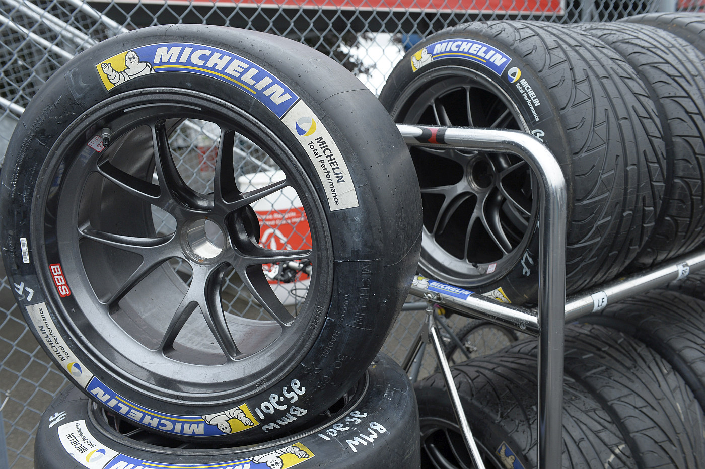
Photo: Michelin Alley
The tyres are the most important single component on a race car (or on any car for that matter). The four tiny contact patches provide the only control forces for the driver to accelerate, brake or change the direction of the car. They are for a car what flight control surfaces are for an aircraft. In order to proper model the behaviour of the car at any phase, the forces generated by the tyres must be accurately modelled.
There are many levels of tyre modelling. Depending on the intended application, the deformations of the tyre can be modelled to analyse the influence of tyre construction on its response. However, this level of tyre modelling is intended for detailed analysis of the tyre itself and is out of the scope of most of lap time simulation packages.
A simpler approach is to create models solely based on actual tyre data. These are mathematical functions that describe tyre behaviour through a well-defined structure and parameters that can be evaluated with the help of regression techniques. The most popular model of this kind is called the Pacejka’s Magic Formula Tyre Model, developed by Hans Pacejka, Egbert Bakker and Lars Nyborg. This model not only provides excellent correlation for lateral and longitudinal forces and self-aligning moment curves, but it does that through coefficients that have clear relationships with typical shapes and magnitude factors of the curves to be fitted.
The model replicates the relationship of lateral force versus slip angle, self-aligning moment versus slip angle and longitudinal force versus slip ratio (the ratio of the difference between the velocity of the tyre at the tread and the forward velocity of the car, and the forward velocity of the car). As this post is just introductory, I will present a brief discussion on the general formulation on pure braking or pure cornering and how the model was created, according to the original paper Tyre Modelling for Use in Vehicle Dynamics Studies (SAE Paper 870421).
The model was developed from the need to represent tyre behaviour from experimental data for vehicle dynamics studies. For that task it is desirable that the parameters involved describe in some way the characteristic quantities of the tyre, such as slip stiffness at zero slip (in the case of cornering forces, this is cornering stiffness, as described here) and peak values of forces and moments.
The Magic Formula is so called because the proposed formulation has no particular physical basis for the structure of the equations in the model. The general shapes of lateral force vs slip angle, self-aligning moment vs slip angle and longitudinal force vs slip ratio curves are presented in figure 1.
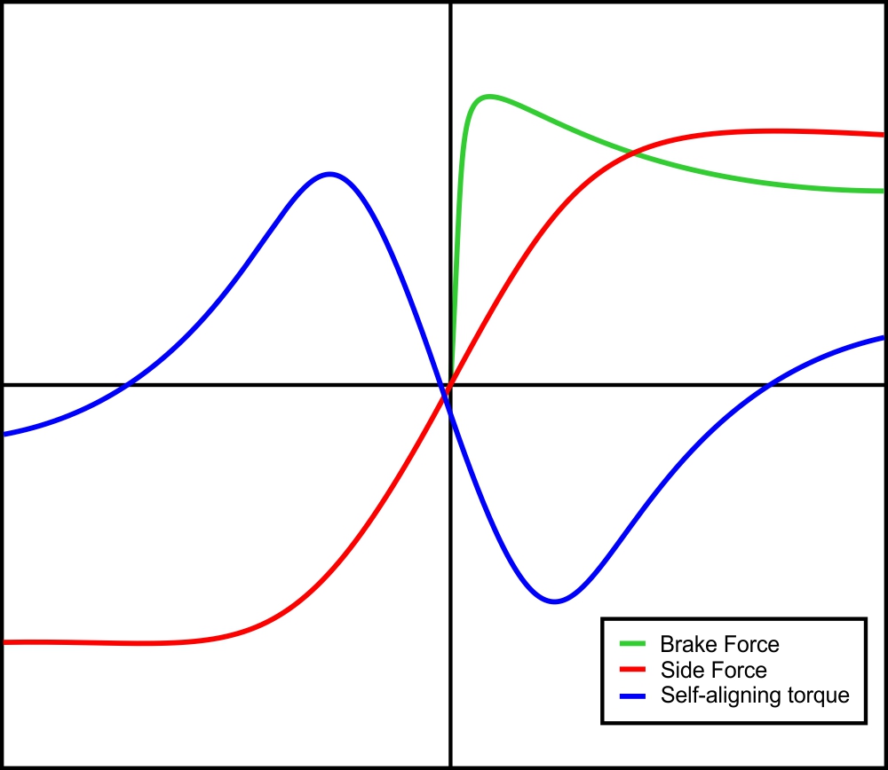
Figure 1. Steady-state tyre characteristics (Bakker, Nyborg and Pacejka, Tyre Modelling for Use in Vehicle Dynamics Studies).
A sine function was used as a first step in trying to match the data.
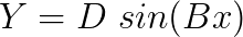
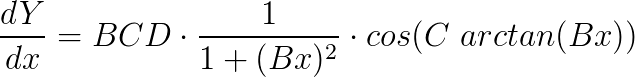
Where Y stands for the force quantity (lateral force, longitudinal force or self-aligning moment) and x is the slip quantity (slip angle or slip ratio). By looking at the formulation, it’s very clear that the coefficient D corresponds to the peak value of force (or moment) in the curve. Now we need to find a relationship for the slip stiffness at zero slip. By definition, the slip stiffness of the curve at any point will be the slope of the curve at that point. From differential calculus, the slope of the curve of a function will be the derivative of that function. So we have:
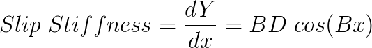
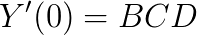
Taking the function at zero slip, we have:

So we have all the coefficients that we need, and we can build a proper model. I’ve set the equations presented above to match a data set from an actual tyre. For confidentiality reasons, the scales of the axes are omitted. The graphs obtained from the model and from the data are shown in figure 2.
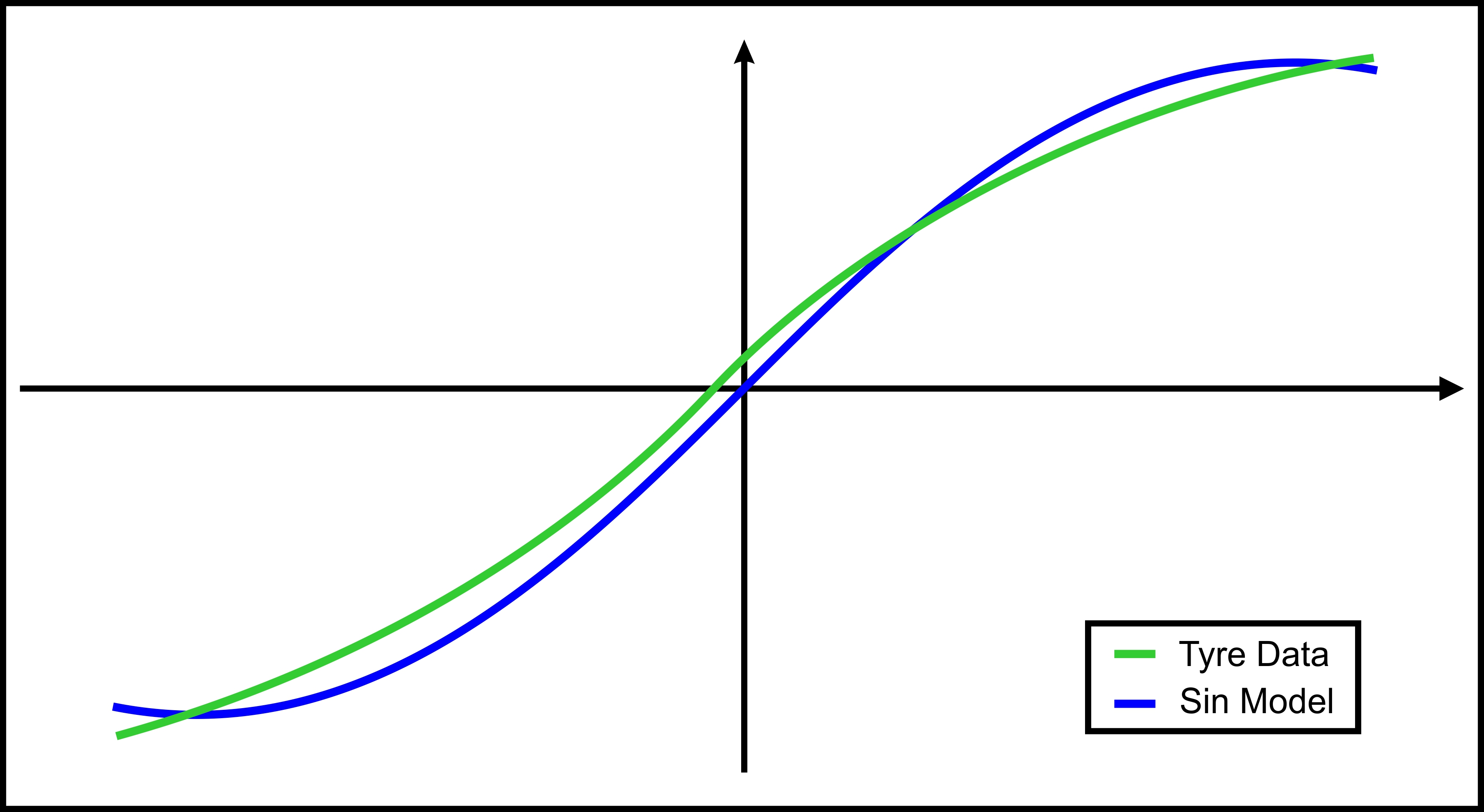
Figure 2. Overlay of plots obtained from an actual tyre and from the sine model.
As observed in figure 2, the sine formulation doesn’t give a good representation once the values of x get larger. To compensate for that, an arctangent term was introduced to the initial formulation, aiming to produce a gradual extension of the x axis. The formulation now becomes:

With this formulation, D still is the peak value of the specific tyre curve. However, the introduction of the coefficient C allows us to have control over the shape of the curve. The value of C also determines the extent of the curve that will be used, and the kind of force quantity that the function will produce. If we take the derivative of Y, we will then have:
This way we can obtain the slip stiffness at zero slip value. Since D is defined by the peak value of the curve and C is fixed by the shape, the parameter B alone is used to control the stiffness. For larger values of x, Y will become  , and the function will look much more like a tyre curve. Figure 3 shows the comparison of the tyre data with the sin(arctan) model.
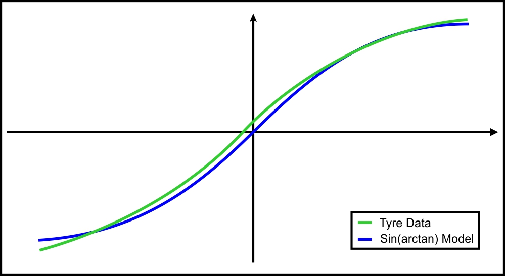
Figure 3. Overlay of plots obtained from an actual tyre and from the sin(arctan) model.
Even though the data fitting got much better, the developers of the model felt the need to accomplish a local compression or stretch of the curve when required. For that, they introduced a fourth coefficient, E. The model then became:

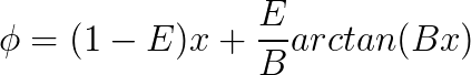
Hence,

The stiffness will then become:


As you can see, the genius of the coefficient E is that it allows us to control the curvature of the function, without affecting the slip stiffness. Figure 4 illustrates the plots of the data from the final formulation and from the actual tyre.
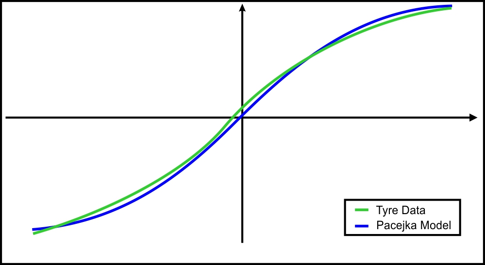
Figure 4. Overlay of plots obtained from an actual tyre and from the sin(arctan(arctan)) formulation.
We now have a formulation with four coefficients that provides a fairly good fit to experimental data of a generic tyre. The original paper in which this model was first described names the coefficients as below:
The coefficients B and D have a direct relation with two characteristic quantities of the tyre (slip stiffness and peak force quantity). So far we assumed that the tyre wouldn’t generate any force at zero slip. This is not always the case, and due to conicity, ply steer and rolling resistance, the tyre curve will not always pass through the origin of the graph. To take that into account, the authors of the paper suggest the implementation of horizontal and vertical shifts (![]() and
and ![]() , respectively) on the model. The formula will then become:
, respectively) on the model. The formula will then become:

This is the general Pacejka’s Magic Formula model for isolated cornering or braking characteristics. The model also takes into account effects of vertical loads and camber, by writing the coefficients and shifts as functions of these parameters. It’s also possible to expand this model for situations with combined braking and cornering. The detailed explanation of these modelling approaches is out of the scope of this introductory post, but I intend to write another more in-depth post about this subject in a near future.
Track Model
Photo: SpeedHunters
A proper track model is key in order to have good correlation from the simulation data. The main function of the track model is to provide a path for the vehicle to follow. However, the path is not the only concern at this stage. All relevant characteristics of the track, such as elevation and banking angle must be analysed, in order to reproduce the effects from these variables on the car model.
We begin with a curvature profile of the track. This can be easily obtained from the data measured on the car. For that, a math channel can be created, according to the following relations:


Where R is the corner radius, V is the vehicle velocity and  is the lateral acceleration of the car, both readily available even on the most basic data acquisition systems. The curvature of the track, k, is the inverse of the corner radius. We can then export the data of a distance plot of curvature, giving a trajectory for the vehicle model to follow. The author Danny Nowlan recommends on his excellent book, The Dynamics of the Race Car, that before exporting the curvature data, we apply a low band pass filter to the signal, set at about 1 Hz, to remove any unwanted corner spikes. Then, when running the first simulation, you should compare the actual curvature with the simulated curvature, just to make sure that no important information was lost with the application of the filter.
The next step is to get elevation information into the model. You might think that this isn’t relevant, but elevations may be a great source of discrepancy between simulated and real-world data. This might be obtained from the GPS data from the car, if available on the data logging system. If this isn’t the case, a more arduous manner would be to use measurements from Google Earth, as suggested by the author Jörge Segers in his book, Analysis Techniques for Race Car Data Acquisition. Figure 5 illustrates.
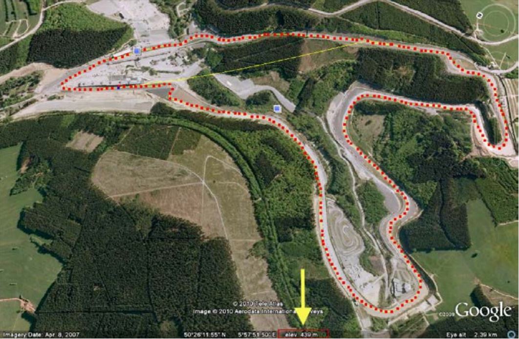
Figure 5. Elevations measurement with Google Earth (Jörge Segers, Analysis Techniques for Race Car Data Acquisition).
Another parameter of great importance is the banking angles at the many points of the track. This can be obtained by creating a math channel with the following equation:
Where  is the vertical acceleration of the car. A good indication that more banking should be added to the track model is when the damper displacements of the actual car are significantly higher than the on the simulated data.
If a transient simulation strategy is used, the track roughness profile must also be provided. This can be done by getting the damper positions signal filtered out to get rid of the low-frequency content, from chassis movements (roll, pitch, and heave). At this point the important thing is to have equal general magnitudes of damper displacements for actual and simulated data, as it’s impossible to get the phasing perfectly right.
All of the above done, it’s possible to implement grip factors to the model, in order to take into account the effects of grip variation from multiple factors (track temperature, level of rubber on the track, dirt, etc.). These may be used to improve local correlation between simulator results and the logged data. However, this should be used with great responsibility, as it can mask problems with the model, resulting with great correlation for a particular setup, but no correlation whatsoever for anything different. If the model was well built until this stage, grip factors should be a fine tweak. The more you need to rely on local grip factors, the more it indicates a problem with either your vehicle model or your lap time simulation routine.
Good Practices for Simulation
Photo: The Yellow Rose’s Pinterest
After putting the car and track models together, the first thing to do is to validate the results against known data. This is done as an iterative process, where one continuously tweaks the model in order to get closer matching between simulated and actual data, to the desired accuracy level. Once this is done, you can use the model/software to start setup evaluations.
The first step after validating the model is to plan a series of what-if scenarios. Lap time simulation is just like a test session done at the computer, so the same testing procedures would apply, with the advantage of much less cost and time. Once the list of desired setup changes is done, a cycle that consists of performing the change, running the simulation and analysing the results will follow.
One important thing to notice is that the changes on the simulation will generally be smaller in magnitude than on the actual car. This will happen because the simulator assumes a driver that has no fear and also, always knows where the maximum grip is. For that reason, a good change is the one which provides a consistent result with no huge spikes.
When analysing the data, you should focus on what the car is doing, as opposed to looking for optimal lap times or strong lap time correlation. One of the main reasons for using lap time simulation is to learn how the car behaves and how it reacts to specific setup changes, so you have to look critically at the obtained set of data, and not rely only on lap times. You should even be more critical with simulated data than with actual information measured on the car, because no simulation model is perfect. A good practice at this point is to rigorously log everything from the simulation, including setup sheets and relevant information input to the model (for example, grip factors).
The changes applied to the setup should be small and deliberate. Also the changes should be applied aiming to improve desired specific traits of the car, as opposed to execute sweep runs or looking after lap times. When you do this, lap times will look after themselves.
Once the virtual testing has been run, a huge database will be available and ready to be cross-referenced with data on the track. When at the track, after the first outing, the data from the car should be overlaid with the simulated data. If the car is working fine, this should be only a sanity check. Between sessions, the data from the simulation will help the engineering team to validate setup decisions, and to remove a good part of the guesswork.
After the visit to the venue, the data from the sessions should be reanalysed against simulated data. This will help to investigate any secondary effects from the changes performed. Then, the real-world data will be used to improve the model, especially in the areas of aerodynamic performance and aeromaps, track bump profiles and tyre model. In categories where vehicle development is allowed, simulations can be run outside the setup ranges of the car, providing results that may motivate changes to the design of specific components or systems.
I hope that this post was enjoyable to you. Hopefully it removed some of the mystery about what occurs in the backstage of professional motorsport, and helped you to better understand the role of simulation, and how much of an invaluable tool it can be when used properly. When good practices are kept, race car simulation is a core part of the race engineering program of any serious professional team.
Did you liked this article? Then please, subscribe to our newsletter below, so that you will never miss a new post around here. Also, please help Racing Car Dynamics by sharing this post on Facebook or on Twitter! See you next time! 😀
KEEP UP TO DATE